Published: July 13, 2017;
20 min read
| Updated: January 14, 2026
Learn how to build a robust credit card fraud detection algorithm in Java using Apache Spark and achieve 98.2% AUC rate.

According to Nilson Report from 2016, $21,84 billion was lost in the US due to all sorts of credit card fraud. On the worldwide scale, the number is even more devastating – $31.310 trillion in total.
Those losses had occurred at every type of credit card (including those, where transactions are protected with a PIN code). Specifically, gross fraud losses for all card-based payment systems on a global scale equaled $6.97 for every $100 of total volume.
And while consumers (especially the online-savvy ones) can easily spot and claim a fraudulent transaction in a matter of hours, it is the banks and the merchants who ultimately shoulder most of the financial burden.
Sure, a fraudulent sale of a $100 pair of jeans does not mean that a retailer loses exactly $100, but a bank will eventually have to reimburse the money to merchant/consumer and issue a new card for the customer (think even more expenses).
Not keeping your backends protected is no longer an option. That’s the lesson all banks have learn well in the recent years. Yet, predicting the fraud before it even occurs, automatically generating the reports and launching preventive systems is something most institutions still need to embrace.
This case study is aimed to demonstrate how you can obtain a forecast for fraudulent card transactions with a 93.5% (or higher) accuracy rate using Java 8 and Apache Spark.
Apache Spark isn’t the only Big Data framework you can use to create a robust credit card fraud detection algorithm. The other common option is a model using clean Python and R.
Yet for this project we chose to stick with Apache Spark for the next major reason:
Spark enables you to conduct all the calculations on a computer cluster – a set of tightly connected computers that function as a single system.
Distributed computing, in this case, will massively speed up the entire process and allow you to conduct simultaneous calculations for different types of problems. Other technologies will not allow to obtain such speed.

Considering that this is a case study, the software program was written for one interesting task from Kaggle.
Here are the details:
We have a dataset of credit card transactions conducted in Europe during two days in September 2014. The initial data is given as a .csv file containing 31 variables within 284.807 transactions. Those variables are:
This dataset may seem nice, but for a real-life experiment it isn’t well-balanced. The percent of fraudulent transactions is only 0.172% of the total number. Yet to make a viable forecast you will need to obtain the highest possible True Positive Rate (TPR) for the classified data and the lowest False Positive Rate (FPR) possible.
If you have similar unbalanced data at hand even the smallest amount of FPR can actually stand for a significant chunk of false positive results within the classification model. Meaning, you will end up verifying a large number of positive cases, which got labelled as fraud instead. Surely, that’s not want you aim for.
The good news is that the problem isn’t new and there are some good solutions to that. In most cases, you can solve it by applying the stratified sampling, so that each stratum is represented by data of the same size.
To identify fraud, I will analyze only certain factors Vi (i=1, 28)and use logistic regression for modeling.
In a nutshell, the process of creating a classification credit card fraud detection model can be summed up in the following points:
Now, let’s get to practicalities!
First, start a Spark session.
Though it’s primarily meant to conduct calculations with the help of a computer cluster, for demos and development, it’s worth running the program locally first:
SparkSession sparkSession=SparkSession.builder()
.master(“local[*]”)
.config(“spark.sql.warehouse.dir”, “file:///c:/tmp/spark-warehouse”)
.appName(“CCFraudsDetection”)
.getOrCreate();
Our data is available as a csv-file, so we need to upload it to the Dataset. Here’s how that’s done:
//–Creating schema of the data in Dataset
StructField[] strField=new StructField[31];
strField[0]=new StructField(“time”, DataTypes.IntegerType, true, Metadata.empty());
strField[29]=new StructField(“amount”, DataTypes.DoubleType, true, Metadata.empty());
strField[30]=new StructField(“class”, DataTypes.IntegerType, true, Metadata.empty());
for (int i=1;i<29;i++){
strField[i]=new StructField(“v”+i,DataTypes.DoubleType, true,Metadata.empty());
}StructType rowSchema = new StructType(strField);
//–Extracting and splitting text from csv-file
Dataset<Row> datasetWithStringRows = sparkSession.read().csv(fileName);//–Removing header and encoding rows in data according schema
Row header = datasetWithStringRows.head();
Dataset<Row> encodedData=datasetWithStringRows.
filter(r->!header.equals(r)).drop(“time”,“amount”).
map(row-> myRowParserToSchema(row,rowSchema),RowEncoder.apply(rowSchema));
Note: myRowParserToSchema (row,rowSchema) is my method of converting the data rows to the specified types.
Considering that a computer cluster will conduct the calculations, we can use the Window class methods to generate sequential numbers for the identification of observations:
encodedData =encodedData.withColumn(“id”,functions.row_number().
over(Window.orderBy(“time”).
partitionBy()));
We don’t have to deal with the multicollinearity problem while building the classificatory as the variables were obtained as a result of PCA.
In this credit card fraud detection project you should also pay attention to the fact that the mean values are zero for the main components, but their variables are different. That’s why we need to avoid the scale effect and standardize the variables.
But first…let’s calculate the main descriptive statistics for non-standardized parameters (so-called raw coefficients) for our model:
Dataset<Row> descriptiveStatistics = data.drop(“id”).describe()
.map(row -> myRowParserToSchema(row,newdescriptivesSchema),
RowEncoder.apply(new DescriptivesSchema));
The describe() method will generate a summary table of the main descriptive statistics for all variables. Yet, as the data would be displayed as String type lines, we will need to cast to row of numeric data types using (new DescriptivesSchema) to account for the numerical data types.
Here’s how this will look:
Descriptive statistics of variables
| Summary | V1 | V2 | . . . | V27 | V28 | Class |
| count | 284807 | 284807 | . . . | 284807 | 284807 | 284807 |
| mean | 0.000 | 0.000 | . . . | 0.000 | 0.000 | 0.0017 |
| stddev | 1.959 | 1.651 | . . . | 0.404 | 0.330 | 0.042 |
| min | -56.408 | -72.716 | . . . | -22.566 | -15.430 | 0.000 |
| max | 2.455 | 22.058 | . . . | 31.612 | 33.848 | 1.000 |
To evaluate the classificatory model, we need two things:
Internally, a matrix within the Dataset is displayed as a set of vectors. That’s why after we execute all the necessary tests and transformations, the selected variables will need to be transformed to a vector representation in the Dataset. In our case, we only do this to calculate the descriptive statistics.
Note: in this technical guide we use only V factors, actual class names, and transaction IDs:
String [] variablesNames=new String[namesOfindependentVars.length+1];
variablesNames[0]=groupingVar;
for(int i=1;i<variablesNames.length;i++){
variablesNames[i]=namesOfindependentVars[i-1];
}
VectorAssembler assemble=new VectorAssembler().
setInputCols(namesOfindependentVars).
setOutputCol(“features”).
transform(data.select(caseIdName,variablesNames)).cache();
To standardize this dataset, we need to deploy the next code:
StandardScaler scaler = new StandardScaler()
.setInputCol(“features”)
.setOutputCol(“scaledFeatures”)
.setWithStd(true)
.setWithMean(false);
StandardScalerModel stdScalerModel = scaler.fit(data);
normalizedData = stdScalerModel.transform(data);
Once we standardize the data, we can split all the transactions into Fraudulent (F) and Honest (H) and work further on more advanced fraud analytics.
Let’s take a closer look on the dataset we had for this model.
Specifically, the model was estimated based on the 70% of F transactions and to ensure accurate data representation we decided to use not less than 5% of honest transactions.Considering that 5% of the total H is much larger than 70% of the total F, we decided to increase the F sample to the size of H.
This approach isn’t new and combines the methods of under-sampling the majority with negative feedbacks and over-sampling the minority with positive feedbacks.
According to Japkowicz research, applying complicated procedures for increasing the sampling dimension will not result in a better model. This statement turned out to be true for our project too.
Specifically, we tested two over-sampling approaches.
In the first approach, we increased the Fraudulent dataset sampling to the size of Honest sampling using the mechanical reproduction of the samples and getting missing observations using the random non-repeat selection process.
In the second one, we accounted only for those transactions, which are situated close to the separation zone between the studied classes. In simple words – only those fraudulent transactions, which were closely alike to the honest ones.
If you need to classify your data into groups and generate random samplings for anomaly detection with Apache Spark, you can use a couple of approaches. For instance, with Dataset class or with the help of SQL:
//- Splitting data to fraudulent and not fraudulent
dataForModel.createOrReplaceTempView(“data_for_splitting”);
Dataset<Row> honestData=sqlContext.sql(“SELECT * FROM data_for_splitting WHERE class=0”);
Dataset<Row> fraudulentData=sqlContext.sql(“SELECT * FROM data_for_splitting WHERE class=1”);//- Splitting data into subsets according to given weights
Dataset<Row>[] fraudulentDataSamples = fraudulentData.randomSplit(new double[]{0.3,0.7});
Dataset<Row>[] reliableData = honestData.randomSplit(new double[]{0.95,0.5});
To conduct a new over-sampling procedure, deploy the following code:
int oldSize = (int)sample.count();
if(oldSize<newSize){
int rest=newSize%oldSize;
int tempSize=newSize–rest;
while(tempSize>0){
newSample= newSample.union(sample);
tempSize-=oldSize;
}//- Getting missing observations using the random non-repeat selection process
if(rest>0){
newSample=newSample.union(sample.sample(false, rest/(double)oldSize));
}
}
Note: Sample stands for the sample you need to increase;
newSize – the number indicating how much larger your sample should become.
Finally, if you have a precise number in mind for your sampling, use this code instead of the last conferment:
sample.createOrReplaceTempView(“sample”);
newSample=newSample.union(sqlContext.sql(“SELECT * FROM sample ORDER BY RAND() LIMIT “+rest));
It’s worth to mention that the samplings you obtain with .sample() or split() commands are closely (but not exactly) corresponding to the size you have indicated. Hence if you need to obtain a very precise sampling, you should rather use SQL methods.
And here’s another problem you may need to solve.
Let’s say you want to conduct over-sampling only for the transactions that are situated close to the separation zone within the studied classes aka the F ones that look really similar to the honest ones.
In this case, before applying the algorithm mentioned above, you’ll need to identify all those transactions for training the model. To do this you should calculate the limits of the major population with the help of minimax criterion.
You can do that by running the next snippet:
VectorAssembler va=new VectorAssembler().
setInputCols(data.drop(Samba).columns()).
setOutputCol(“features”);
Dataset<Row> datasetWithFeatures = va.transform(data).
select(nameOfGroupingVar,”features”).cache();
RelationalGroupedDataset groupedByClass = datasetWithFeatures.
groupBy(data.col(nameOfGroupingVar));
Vector upperLimits=(Vector)groupedByClass.
agg(functions.max(“features”)).
agg(functions.min(“max(features)”)).
head().get(0);
Vector lowerLimits=(Vector)groupedByClass.
agg(functions.min(“features”)).
agg(functions.max(“min(features)”)).
head().get(0);
Using the calculated criteria, we have selected rows that correspond to it for the set number of variables. The code below demonstrates how this filter can be implemented:
Dataset<Row> filter = initialDataForOversampling.filter(row->{
Vector v = (Vector)row.get(2);
int counter=0;
for(int i=0;counter<numberOfPositiveChecks&&i<v.size();i++){
if(v.apply(i)<upperLimits.apply(i) && v.apply(i)>lowerLimits.apply(i)){
counter++;
}
}
return (counter>=numberOfPositiveChecks);
});
Note: numberOfPostiveChecks stands for the minimal number of variables that will match the filter criteria, which is required to gather the data for over-sampling.
So what do we have so far?
For model estimation we have gathered a sampling of 28408 observations that include:
For testing, we used a 95% honest transaction sampling (270574 cases) and 30% of fraudulent ones (148 cases). That’s the data that wasn’t accounted for when estimating the classifier model.
Next, we also used over-sampling to form the sub-sampling of fraudulent transactions. Specifically, we did the over-sampling using the next proportion (172:100,000). That was done for a reason of course. The data we had didn’t quite account for TP (true positive) and FP (false positive) cases, so we re-created the proportion between TP and FP, which we would have had with the full data.
Note: The over-sampling was done using the same algorithm as we applied for the training model without a filter.
To answer the question of how to detect credit card fraud with Spark, we need to specifically look into the process of estimation and testing the classifier model. In our case, for model estimation we used non-filtered sampling.
For the classification itself, we used a logistic regression model. To estimate it, the next code was deployed:
LogisticRegressionModel lRegrModel = new LogisticRegression()
.setLabelCol(“class”)
.setFeaturesCol(“scaledFeatures”)
.setPredictionCol(“forecast”)
.setProbabilityCol(“probability”)
.setStandardization(false)
.setMaxIter(40)
.fit(trainingData);
To calculate the model parameters, you should deploy:
Vector ModelCoefficients = lRegrModel.coefficients();
double intercept=lRegrModel.intercept();
So now we have the next prediction for the training sample:
LogisticRegressionTrainingSummary trainingSummary = lRegrModel.summary();
Dataset<Row> predictedClasses =trainingSummary
.predictions()
.select(“id”,“class”,“probability”,“forecast”);
predictedClasses.show(false);
In the table below you can see how the predictions of fraudulent cases on the training sample will look:
Predictions of fraudulent cases on the training sample
| ID | Class | Probability | Forecast |
| 42550 | 1 | [2.1161498101003494E-39,1.0] | 1.0 |
| 119714 | 1 | [0.7752566613777615,0.22474333862223864] | 0.0 |
| 108761 | 0 | [0.8458327697467396,0.15416723025326037] | 0.0 |
| 192583 | 1 | [2.4208133100008088E-14,0.9999999999999758] | 1.0 |
| 61525 | 0 | [0.9963678126766196,0.0036321873233805435] | 0.0 |
| 102442 | 1 | [1.1370856010735598E-23,1.0] | 1.0 |
| 9359 | 0 | [0.9851127033549458,0.014887296645054188] | 0.0 |
| 42857 | 1 | [2.268814783287015E-29,1.0] | 1.0 |
| 36953 | 0 | [0.8892984969468882,0.1107015030531118] | 0.0 |
| . . . | . . . | . . . | . . . |
Some quick comments on the table data.
Here we are dealing with binary classifiers. So our job is to build a model that would estimate the function, which can evaluate the differences between the classes, and then set a threshold that separates Class 0 from Class 1.
Here’s a quick example of how a classifier that would evaluate the differences between two classes will look:
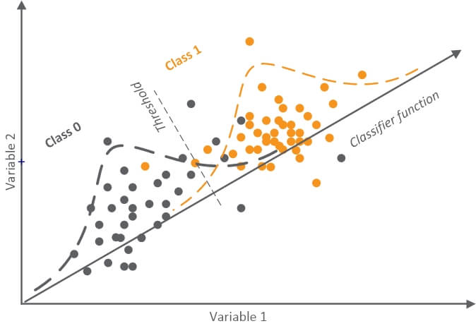
According to this graphic, the classifier function can be interpreted as a vector located on the coordinate space, whose axes are independent variables. Specifically, the vector should be built in such way that its position to shows the most differences between classes.
As you can see, a classifier can be identified as a new vector that is situated in the space indicated by the initial variables. Those variables should convey the majority of differences between classes.
By modifying the separation threshold between the two classes, we modify the ratio of correctly identified cases (True Positive Rate) from Class 1 (fraudulent transactions) and the ratio of incorrectly classified cases (False Positive Rate) from Class 0 (honest transactions).
(As you remember, the problem here is to balance between TPR and FPR.)
I should mention that input variables typically do not create a coordinate space of space of orthogonal vectors. Besides, to obtain clear classification functions, as in this picture, root transforms are often applied.
To analyze the quality of binary classification and to choose the optional threshold, Confusion Matrices and ROC-curves (receiver operating characteristic curves) are typically used. Depending on the classifier’s quality, a ROC-curve will correspond to either of the following schemes:
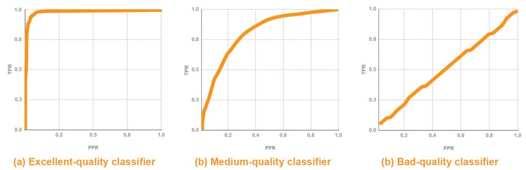
The bottom left point on the curve corresponds to the threshold, which indicates that all observations should be classified as Class 0. The upper right point, on the contrary, indicates a threshold for observations classified as Class 1.
Within a well-balanced distribution for both classes, the optimal threshold will correspond to the point on the curve that is situated the closest to the upper left corner on the graphic. Specifically, a point with (0;1) coordinates.
ROC-curve at Pic a. shows an excellent classifier.
Picture b. shows a medium-quality classifier as the balance point between TRP and FRP here is situated quite far from the upper left corner.
Finally, the last graphic shows a case when a classifier matches some random choice, meaning that his ability to determine the correct class for an observation is close to 0.5.
Here’s the next important point. Mind the Array Under Curve (AUC) index. It will tell you how good your classifier is.
A ROC-curve at Pic a. has an AUC ranging from 0.9 to 1 and the ROC-curve at pic c. has AUC≈0.5.
One of the cool Spark use cases is that you can generate ROC curves rather efficiently. First, you will need to obtain an instance of BinaryLogisticRegressionSummary class, and then calculate the coordinate points on the curve:
BinaryLogisticRegressionSummary binarySummary = (BinaryLogisticRegressionSummary) trainingSummary;
Dataset<Row> roc =binarySummary.roc();
Roc.show(false);
ROC characteristics
| FPR | TPR |
| 0.0 | 0.0 |
| 4.224162207828780 | 0.8096310898338496 |
| 0.008800337932976627 | 0.8824274852154322 |
| 0.01823430019712757 | 0.910377358490566 |
| 0.02823148408898902 | 0.9160095747676711 |
| 0.03815826527738665 | 0.9216417910447762 |
| 0.04787383835539285 | 0.9356519290340749 |
| 0.05780061954379048 | 0.94128414531118 |
| . . . | . . . |
A ROC-Curve for such classifier can be shown graphically the following way:
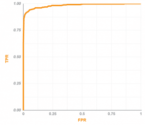
The AUC for this curve is 0.9844, meaning that the classifier is excellent.
To calculate this AUC number with Spark, you’ll need to deploy the next code:
double AUC=binarySummary.areaUnderROC();
System.out.println(“AUC=”+AUC);
Now, let’s take a look at how the threshold value impacts the results obtained from our classification with the help of confusion matrices.
To get the data with Spark, we’ll have to re-calculate the intercept in the cycle for different threshold values in the model we already have:
LogisticRegressionModel lrModel = lRegrModel.setThreshold(threshold);
Let’s calculate the forecast for a modified model:
Dataset<Row> predictions = lrModel.
evaluate(testSample).
predictions();
And compute statistics for the confusion matrices:
Dataset<Row> classesInFactVsPredicted = predictedClasses.select(“class”,”forecast”);
Dataset<Row> positiveInfact = classesInFactVsPredicted.
where(classesInFactVsPredicted.col(“class”).equalTo(1));
Dataset<Row> negativeInfact = classesInFactVsPredicted.
where(classesInFactVsPredicted.col(“class”).equalTo(0));
long[][] confusionMatrix=new long[2][2];//- Computing number of true positive predictions
confusionMatrix[0][0] = positiveInfact.
where(classesInFactVsPredicted.col(“forecast”).
equalTo(1)).count();//- Computing number of false negative predictions
confusionMatrix[0][1] = positiveInfact.
where(classesInFactVsPredicted.col(“forecast”).
equalTo(0)).count();//- Computing number of false positive predictions
confusionMatrix[1][0] = negativeInfact.
where(classesInFactVsPredicted.col(“forecast”).
equalTo(1)).count();//- Computing number of true negative predictions
confusionMatrix[1][1] = negativeInfact.
where(classesInFactVsPredicted.col(“forecast”).
equalTo(0)).count();
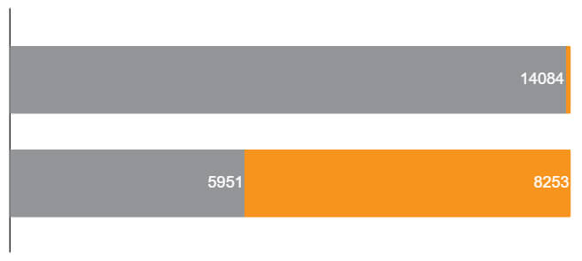
The obtained data can be visualized the following way:
Confusion matrix for threshold=0.05
| Actual class | Predicted class | |
| Fraudulent | Honest | |
| Fraudulent (recall) | 14084 | 120 |
| 99.16% | 0.85% | |
| Reliable (recall) | 5951 | 8253 |
| 41.90% | 58.10% | |
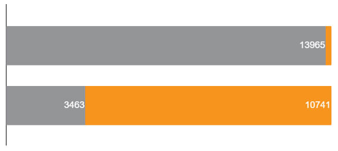
Confusion matrix for threshold=0.1
| Actual class | Predicted class | |
| Fraudulent | Honest | |
| Fraudulent (recall) | 13965 | 239 |
| 98.32% | 1.68% | |
| Reliable (recall) | 3463 | 10741 |
| 24.38% | 75.62% | |
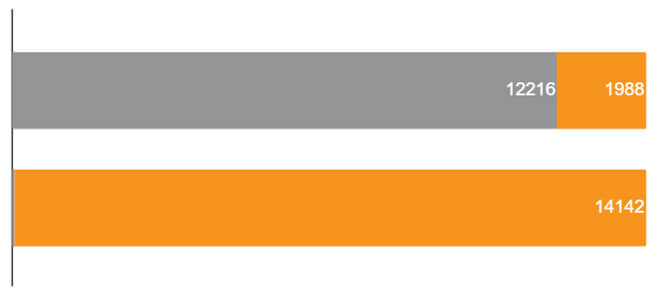
Confusion matrix for threshold=0.9
| Actual class | Predicted class | |
| Fraudulent | Honest | |
| Fraudulent (recall) | 12216 | 1988 |
| 86.00% | 14.00% | |
| Reliable (recall) | 62 | 14142 |
| 0.44% | 99.56% | |
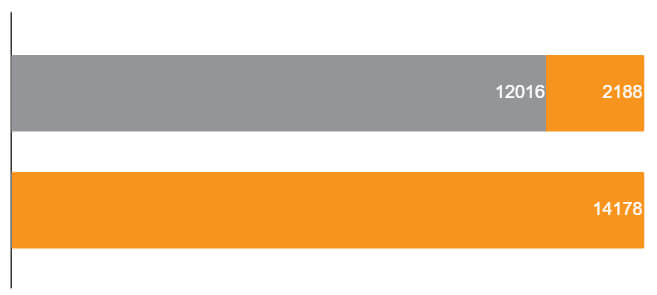
Confusion matrix for threshold=0.95
| Actual class | Predicted class | |
| Fraudulent | Honest | |
| Fraudulent (recall) | 12016 | 2188 |
| 84.60% | 15.40% | |
| Reliable (recall) | 26 | 14178 |
| 0.18% | 99.82% | |
Let’s sum up one of the important data analytics techniques for fraud detection in this case.
When developing a classifier for identifying the unlikely events, you need to aim for the high value of TRP) and low value of FPR. As the tabs above demonstrate – as the threshold increases, the number of identified fraudulent transactions reduces. Yet, you also reduce the FPR number.
Considering that the model estimation was conducted with a credit card processing sample that had an equal amount of fraudulent and honest transactions, an optimal classifier should correspond to the ROC point in the upper left corner (point 0;1).
For this fraud detection model, the optimal threshold turned out to be 0.753. This optimal number was estimated using F-Measure:
Dataset<Row> thresholdVsF=binarySummary.precisionByThreshold();
double maxF = thresholdVsF.select(functions.max(“F-Measure”))
.head()
.getDouble(0);
double bestThreshold = thresholdVsF
.where(thresholdVsF.col(“F-Measure”).equalTo(maxF))
.select(“threshold”)
.head();
This threshold confusion matrix for a training sample is shown below:
Confusion matrix for threshold=0.753
| Actual class | Predicted class | |
| Fraudulent | Honest | |
Fraudulent (recall) | 12534 | 1670 |
| 88.24% | 11.76% | |
Reliable (recall) | 126 | 14078 |
| 0.89% | 99.11% | |
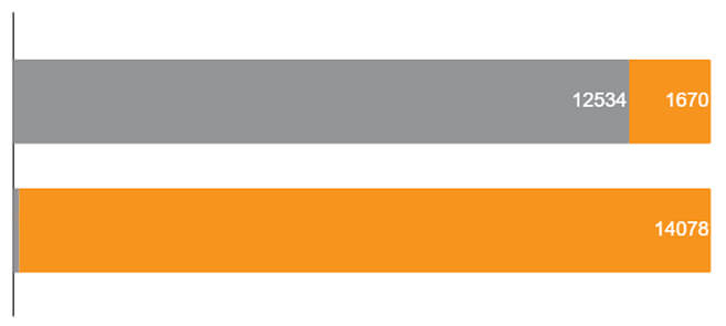
What we managed to obtain is a recall level equal to 88.24% and a 99% precision rate.
If we take the mean value to evaluate the system’s performance, the forecast accuracy will be 93.5%. Impressive protection and monitoring service quality for any bank, right?
For the final model testing, we used a classifier with an AUC = 0.9837. It’s of the same quality as we used for the training sample.
The forecast accuracy can be viewed below:
Confusion matrix for testing sample
| Actual class | Predicted class | |
| Fraudulent | Honest | |
| Fraudulent (recall) | 404 | 62 |
| 86.7% | 13.3% | |
| Reliable (recall) | 514 | 269594 |
| 0.19% | 99.81% | |
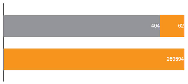
And if we are talking numbers so much…. let’s have a look on how much money we just saved some lucky “bank”.Here’s some awesome news – to identify 87% of all frauds, we need to check just 918 transactions out of 270.000 total. Easy-peasy, right?
During the analyzed two days, the total value of all fraudulent transactions was 60,128 euro. Considering that the fraud levels remain the same, that’s close to 1 million euro per month!
At the same time, we couldn’t identify around 7.600 euro worth of fraud transactions. But if you need to increase the percent of identified frauds for the very same classifier, you can set another threshold. The one that would cost you less to deploy compared to the damaged caused by non-identified frauds.
Remember the second approach we used for training our model?
That time when we used over-sampling to fraudulent transactions which were closely alike to the honest ones? Specifically, we added observations that were similar by 5%, 10%, 20%, 30% and 40% of variables.
When testing a filter with a 30% variable and above, the results were not as accurate as in the testing sample. Filters of 30% and less were closely alike to the results obtained without using filters in over-sampling.
In this case study, we used a logistic regression model. But you can also obtain close results with Discriminant Analysis. But you will then need to do more coding, as this method cannot be deployed in Apache Spark.
To draw the final line – this classifier model can be efficiently used to determine all sorts of fraudulent credit card transactions, happening both online and offline. The particular appeal here is that the big data is getting real’ big and is expected to grow exponentially further on. Cluster computing can be the answer to analyzing huge chunks of data simultaneously and at an impressive speed.
Fraud detection is just one example of how a financial institution can benefit from such model. A cluster computer can work on multiple problems at once and analyze compliance risks associated with a certain transaction; generate reports and recognize abnormal trading patterns early on.
You can also deploy a similar model for advanced customer segmentation. Specifically, you’ll be able to group theirs into distinct segments that share common demographics, daily transactions, and interactions with the bank. Next, you can level up your marketing campaigns to target those groups with highly personalized offers.
If you’d like to learn more about the benefits of big data services for your business, don’t hesitate to get in touch with the Romexsoft.
Java offers a robust platform for building credit card fraud detection systems. The article from Romexsoft demonstrates how Java can be integrated with various algorithms and tools to detect and prevent fraudulent transactions. Java's versatility and scalability make it an ideal choice for developing sophisticated fraud detection applications.
A fraud detection system's design encompasses several components, including data preprocessing, feature extraction, and the selection of appropriate algorithms. The system should be capable of analyzing vast amounts of transaction data in real-time, identifying patterns, and flagging suspicious activities. The design should also consider factors like system scalability, real-time processing capabilities, and integration with other systems.
Credit card fraud detection relies on a combination of algorithms to identify suspicious activities. Some of the popular algorithms include Decision Trees, Neural Networks, Logistic Regression, and Random Forests. The choice of algorithm depends on the nature of the data, the specific requirements of the detection system, and the desired accuracy levels.
Developing a Java-based detection app involves several steps. First, gather and preprocess the transaction data. Next, extract relevant features from this data that will aid in detection. Then, choose and implement the appropriate fraud detection algorithms. Finally, integrate the app with the existing transaction systems, ensuring real-time processing and timely alerts for any suspicious activities.